PV Module Shading in Utility-Scale Solar Plants: Real Impact on PR, CUF and Energy Yield
Shading is one of the most underestimated performance loss categories in operating solar power plants. Unlike inverter faults or grid curtailment, shading losses are silent — they depress your Performance Ratio (PR) and Capacity Utilisation Factor (CUF) gradually and predictably, often without triggering a single alarm on your SCADA system.
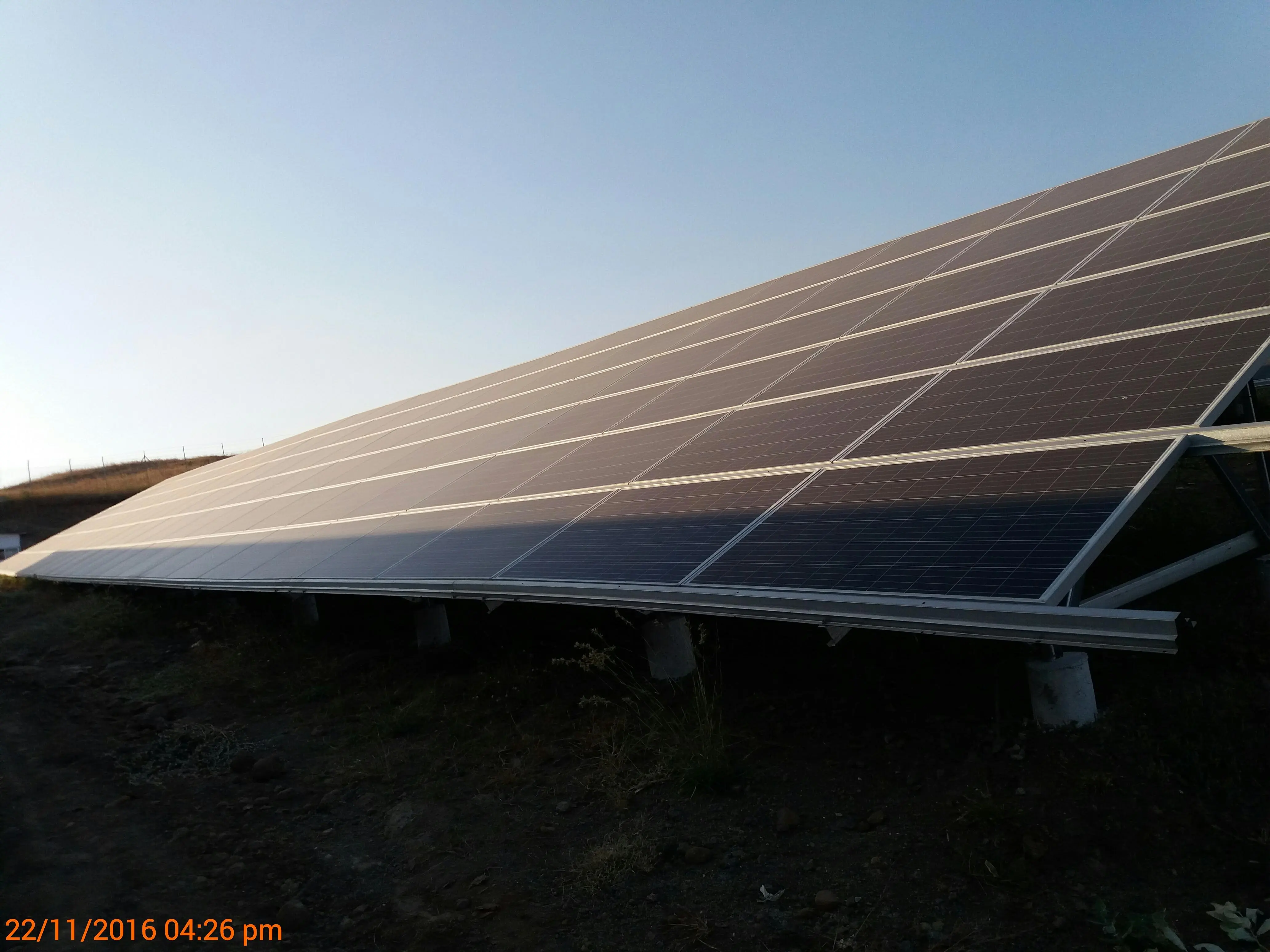
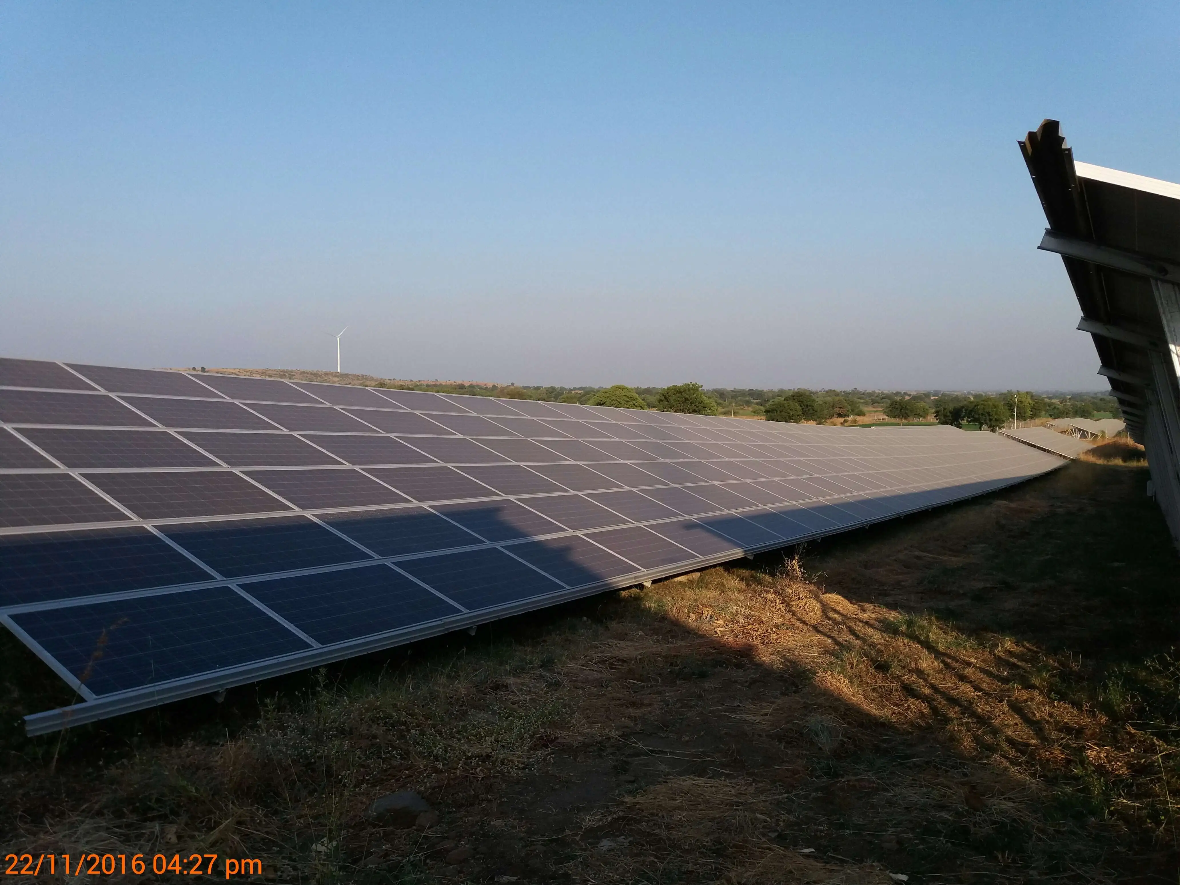
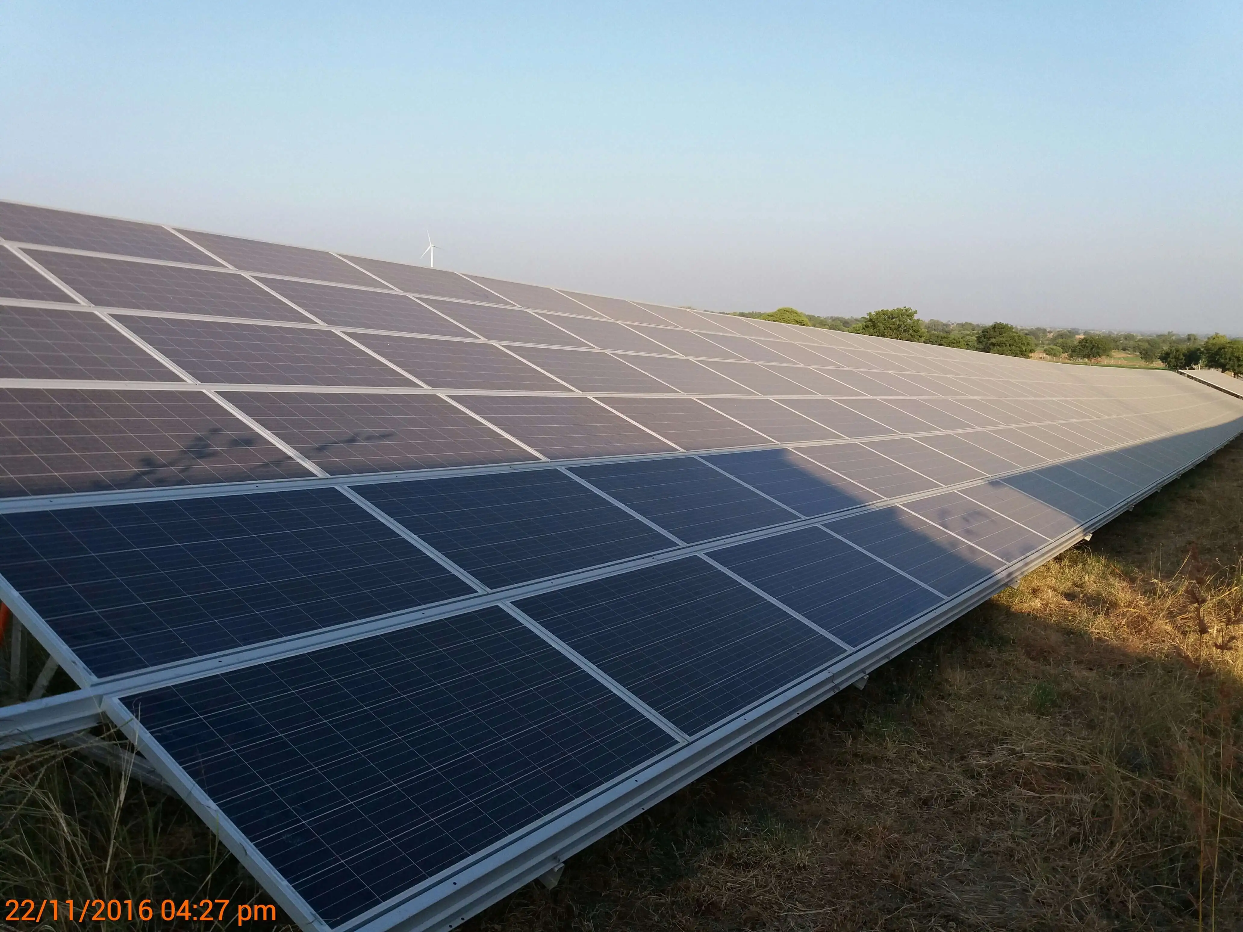
This article is grounded in field observations from a 15 MWp ground-mounted plant in Rajasthan, India, using 265 Wp polycrystalline modules (HT60-156P-265, 24 modules per string), supported by real 15-minute interval SCADA data and site photographs across multiple plant types. The shading mechanisms, electrical consequences, and performance impacts described here apply broadly to utility-scale and commercial ground-mounted solar plants worldwide.
Why Shading Hits Harder Than You Expect
The physics of shading in a series-connected PV string is fundamentally non-linear. When cells in a string are shaded, they cannot source the full operating current of the remaining unshaded modules. Left unprotected, those reverse-biased cells would dissipate power as heat — a condition that accelerates cell degradation and can lead to permanent hotspot damage.
To prevent this, every crystalline silicon module is fitted with bypass diodes inside the junction box. A standard 60-cell module — like the HT60-156P-265 used at this plant — contains three bypass diodes, one protecting each group of 20 cells (one submodule). When even a narrow band of cells within a submodule is shaded, the diode conducts and short-circuits that entire 20-cell section.
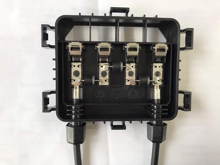
The electrical consequence is disproportionate to the shaded area. When a bypass diode conducts, it removes approximately one-third of the module's voltage contribution from the string — though the actual loss varies with operating irradiance, module temperature, string current, and the MPPT operating point. On a string of 24 modules (Vmp ≈ 31.5 V per module, string Vmp ≈ 756 V at STC), the activation of one bypass diode on a single module removes roughly that module's submodule voltage from the total string voltage. When multiple modules on the same string are simultaneously shaded, the inverter MPPT must re-track to a shifted operating point — and on strings where shading creates a multi-peak IV curve, some MPPT algorithms settle on a local rather than global maximum, further amplifying the loss.
Types of Shading Encountered in Operating Solar Plants
Not all shading sources behave the same way electrically or operationally. Understanding the source determines how you detect it, quantify it, and address it. In ground-mounted utility-scale and commercial plants, five shading types appear most frequently.
1. Inter-Row Self-Shading
This is the most common shading type at utility-scale ground-mounted sites. It occurs when one row of a fixed-tilt array casts a shadow onto the adjacent row during low solar elevation angles — typically in the early morning, late afternoon, and throughout winter months at higher latitudes. Which row receives the shadow depends on site geometry and row orientation.
The shadow length is governed by direct geometry: shadow length = H ÷ tan(solar elevation angle), where H is the height of the module's top edge above ground. At solar elevations below 20°, shadows extend several metres beyond the front edge of each table row. The ground coverage ratio (GCR) chosen at design stage determines how quickly inter-row shading onset occurs as the sun descends through the afternoon.
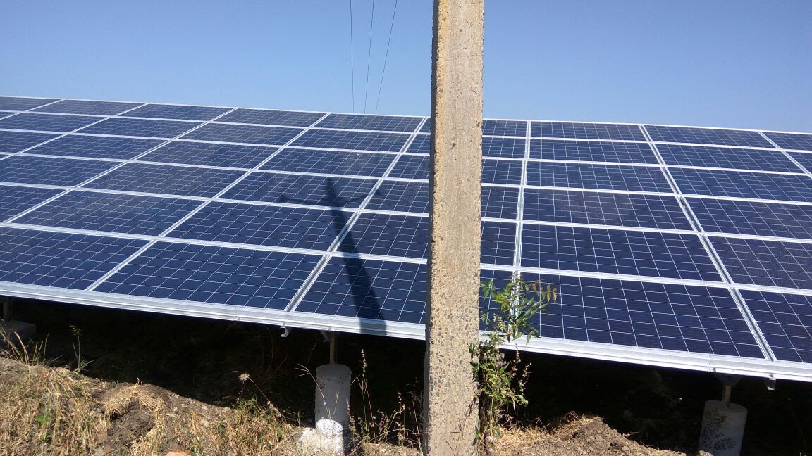
2. External Obstruction Shading — Utility Poles and Overhead Lines
At many utility-scale sites, pre-existing infrastructure cannot be relocated before commissioning. Distribution poles, overhead LT or HT lines, telecom towers, and boundary structures inside or immediately adjacent to the array boundary create moving, directional shadows throughout the day.
Unlike inter-row shading — which affects module rows uniformly — pole shadows are narrow and diagonal. They cross multiple string boundaries simultaneously as the sun moves. A single concrete utility pole can affect strings in two or more adjacent table sections depending on sun azimuth. Because the shadow angle and length change continuously through the day, identifying the affected strings requires cross-referencing string monitoring timestamps with solar position data.
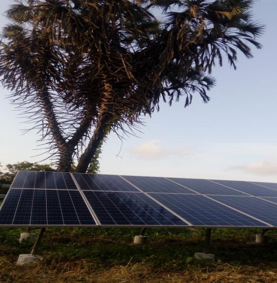
3. Boundary Tree and Peripheral Vegetation Shading
Trees at or beyond the array boundary are a persistent shading source at sites in tropical, subtropical, and temperate agricultural regions worldwide. Unlike inter-row shading, tree shadow has a soft, diffuse boundary — partial penumbra shading, rather than a crisp geometric line. This diffuse character makes tree shading harder to see clearly in string-level current data, because the irradiance reduction is gradual rather than stepped.
At sites in Southeast Asia, Sub-Saharan Africa, South Asia, and Latin America, boundary trees are often mature pre-existing vegetation that falls outside the cleared project footprint. Their shadow trajectory across the array changes with season and sun declination, meaning the affected strings and modules shift month to month.
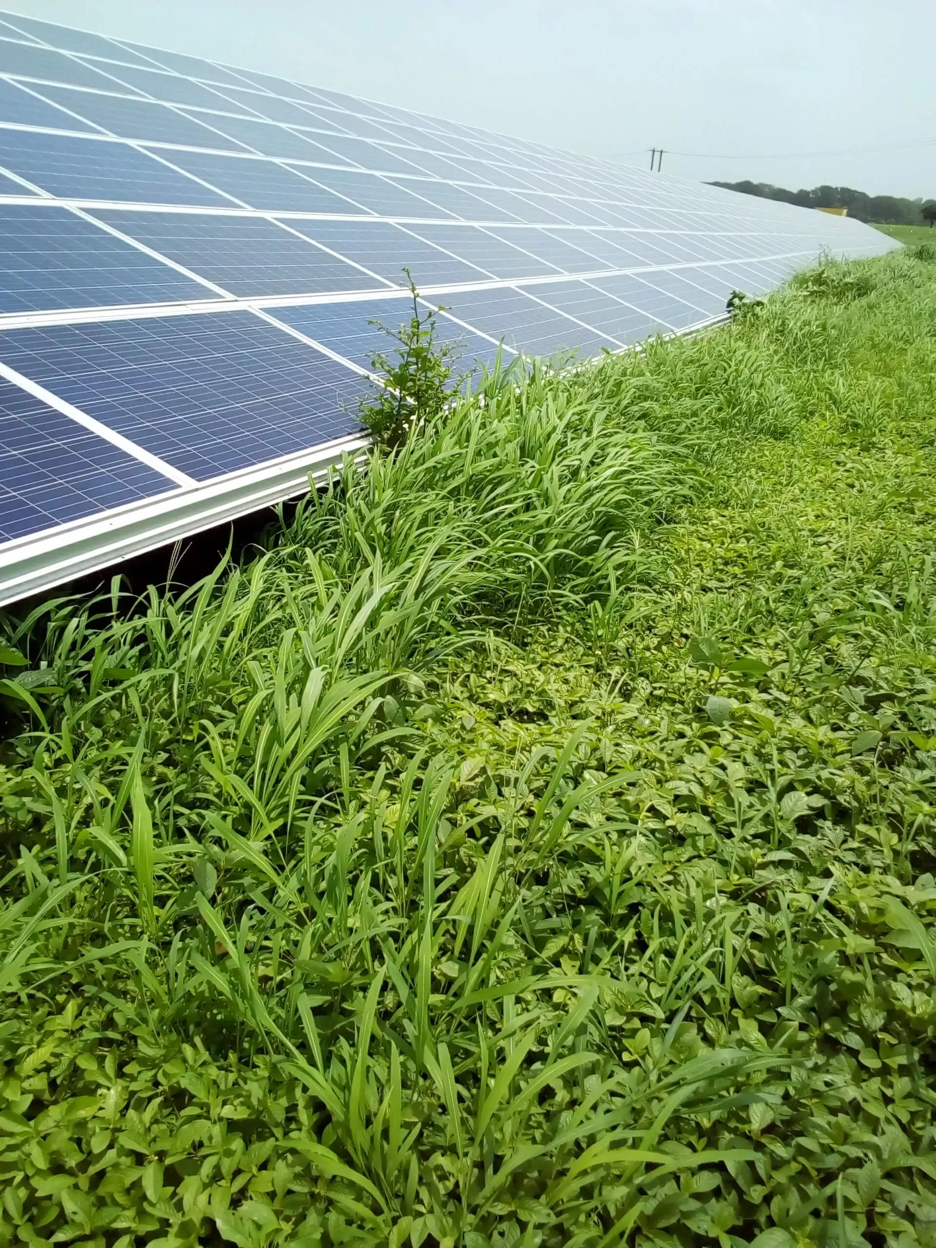
4. Vegetation Growth and Weed Encroachment
In tropical and subtropical climates, weed and shrub growth during monsoon or rainy seasons can reach the lower edge of module frames within weeks if vegetation management schedules slip. Unlike geometric shadows, vegetation shading is irregular and patchy — it affects different cells on different modules within the same string, creating complex mismatch conditions that standard string-level monitoring may not clearly flag.
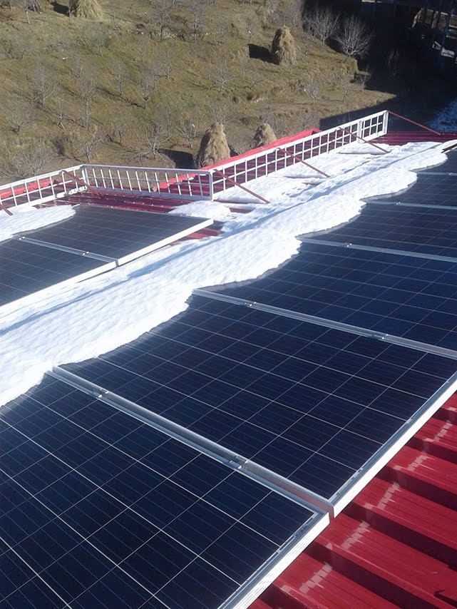
5. Snow and Ice Coverage (High-Altitude and Cold-Climate Sites)
For plants operating at altitude or in cold climates — Himalayan hillside installations, northern European ground arrays, or high-altitude sites in Chile, the US Rockies, or Central Asia — snow accumulation is a seasonal shading concern. Partial snow coverage often creates severe mismatch losses relative to uniformly covered modules.
How Shading Appears in Your Performance Data
The most operationally important characteristic of shading losses is that they are time-correlated and repeatable — they follow the sun. This predictability is both their signature and their primary diagnostic tool.
At the 15 MWp plant documented here, 15-minute interval data captured the following pattern on 22 November 2016, a clear winter day. The data compares an unshaded reference scenario against the measured shaded output for an affected ~800 kWp inverter block. The plane-of-array (POA) irradiance data showed stable irradiance conditions consistent with a clear day — strongly indicating shading as the dominant cause.
15-Minute Interval Shading Loss Data — Full Afternoon Window
| Time (IST) | POA (W/m²) | DC — No Shading (kW) | DC — With Shading (kW) | DC Loss (kW) | DC Loss (%) | AC — No Shading (kW) | AC — With Shading (kW) | AC Loss (kW) |
|---|---|---|---|---|---|---|---|---|
| 15:00 | 732.6 | 478 | 454.1 | 23.9 | 5% | 463.1 | 439.9 | 23.2 |
| 15:15 | 697.3 | 459 | 436.1 | 22.9 | 5% | 445.6 | 423.3 | 22.3 |
| 15:30 | 649.8 | 425 | 403.8 | 21.2 | 5% | 411.8 | 391.2 | 20.6 |
| 15:45 | 602.3 | 394 | 374.3 | 19.7 | 5% | 382.9 | 363.8 | 19.1 |
| 16:00 | 541.2 | 352 | 323.8 | 28.2 | 8% | 342.3 | 314.9 | 27.4 |
| 16:15 | 485.9 | 319 | 293.5 | 25.5 | 8% | 310.9 | 286 | 24.9 |
| 16:30 | 436.3 | 281 | 258.5 | 22.5 | 8% | 272.3 | 250.5 | 21.8 |
| 16:45 | 380.3 | 243 | 223.6 | 19.4 | 8% | 235.1 | 216.3 | 18.8 |
| 17:00 | 314.1 | 195 | 165.8 | 29.2 | 15% | 187.5 | 159.4 | 28.1 |
| 17:15 | 254.2 | 158 | 134.3 | 23.7 | 15% | 153.4 | 130.4 | 23.0 |
| 17:30 | 207.3 | 118 | 100.3 | 17.7 | 15% | 114.3 | 97.2 | 17.1 |
| Window Total | — | — | — | — | — | 829.8 kWh | 768.2 kWh | 61.6 kWh |
| kWh values = sum of 15-min interval power readings × 0.25 h per interval. | ||||||||
Quantifying the Full-Day Impact on PR and CUF
The Performance Ratio as defined by IEC 61724-1 compares measured AC energy output against the reference yield derived from plane-of-array (POA) irradiance and installed DC capacity:
PR = EAC / (HPOA × PSTC)
Where EAC is measured AC energy (kWh), HPOA is daily plane-of-array insolation (kWh/m²), and PSTC is nameplate DC capacity (kWp). Source: IEC 61724-1:2021.
Shading directly reduces EAC — the numerator — while the denominator remains unchanged. The full-day PR and CUF impact from the field data at this plant, calculated for the affected ~800 kWp inverter block, is as follows:
| Metric | Without Shading | With Shading | Delta |
|---|---|---|---|
| Daily AC Energy (~800 kWp block) | 4,433.9 kWh | 4,372.3 kWh | −61.6 kWh |
| Performance Ratio (PR) | 77.83% | 76.75% | −1.08 percentage points |
| Daily CUF | 23.09% | 22.77% | −0.32 percentage points |
| Shading loss as % of daily generation | — | — | 1.39% |
This data represents a single clear winter day on one inverter block. It is presented as a field-measured illustration of how afternoon shading registers in PR and CUF calculations, not as a basis for annual yield extrapolation. The magnitude of seasonal impact depends on the number of affected blocks, the frequency of clear-day shading events, and site-specific geometry — all of which require full plant-level analysis across a representative dataset to quantify defensibly.
Use your plant's CUF calculator and PR calculator on the shaded hours alone — isolating just the 15:00–17:30 window, for example — to quantify your intra-day shading loss precisely rather than relying on diluted daily averages.
How to Identify Shading Loss in Your PR Reports
Most plant-level MIS reports aggregate performance data into daily or monthly averages, which can mask time-correlated shading signatures. A practical diagnostic approach using standard 15-minute interval SCADA data works as follows.
- Plot intra-day power against POA irradiance on clear days. Without shading, the AC or DC power-to-irradiance ratio should remain approximately stable through the day, adjusted for temperature. A consistent dip in this ratio during a specific time window — particularly during low sun elevation hours — is a shading indicator.
- Compare string currents between affected and unaffected rows. On plants with string-level monitoring, strings in the rows that receive shadow will show lower current during the shading window compared to strings in rows that remain unshaded. Which rows are affected depends entirely on site geometry — identify this from a site survey, not from assumptions about row position.
- Check whether the dip is sun-angle dependent. If the PR drop begins earlier in winter months than in summer and correlates with a specific sun elevation threshold, inter-row or obstruction shading is almost certain.
- Classify the loss correctly in your PR waterfall. Shading loss is an irradiance-related loss — it reduces effective irradiance at the module surface. Report it separately from soiling, thermal, wiring, and inverter losses to enable accurate root-cause attribution.
Corrective Actions by Shading Type
Once shading is confirmed and quantified, the corrective action depends entirely on the shading source.
- Inter-row shading from fixed-tilt design: This is a layout constraint established at design stage through GCR selection. At an operating plant, re-routing strings to group shaded and unshaded modules into separate strings — rather than mixing them within the same string — can reduce mismatch losses, though it requires DC rewiring work. The economic case must be assessed against the measured loss magnitude.
- External obstructions (poles, towers, billboards): The primary action is to pursue relocation or removal through the relevant authority. Where that is not achievable in the near term, documenting the shading loss with measured SCADA data is essential for internal performance reporting and for any commercial or contractual discussions regarding generation shortfall.
- Boundary trees: At sites where tree trimming or removal is permissible, scheduled canopy management directly recovers generation. Where removal is not possible, the loss should be quantified and carried as a known site-specific deduction in performance benchmarking.
- Vegetation and weed growth: This is the most operationally tractable source. Shortening vegetation clearance intervals during peak growing seasons eliminates this loss category directly. Specifying maximum allowable vegetation height in O&M contracts is standard at well-managed sites.
- Snow coverage: Steeper tilt angles during design accelerate natural clearing. Anti-soiling coatings on module glass help marginally. Manual clearing protocols are justified at high-altitude plants where snow events are frequent and generation loss is material.
Conclusion
Shading is not a single problem — it is a family of site-specific conditions that each require field-level investigation rather than generic mitigation advice. The 15-minute interval field data from this 15 MWp plant demonstrates measurable, quantifiable impacts: a 1.08 percentage point daily PR drop, a 0.32 percentage point daily CUF reduction, and a 7.4% energy loss during the shaded afternoon window — all from a single winter day's afternoon inter-row and obstruction shading.
What makes shading particularly costly over a plant's life is that it is predictable. It follows the sun. If your afternoon PR is consistently below your morning PR on clear days — without fault alarms, without curtailment, without soiling — shading deserves to be the first thing you investigate, not the last.
Use your 15-minute interval SCADA data, cross-reference it with solar position data, and calculate your PR and CUF on a sub-daily basis. That is where shading hides — and that is precisely where you will find it.
Frequently Asked Questions
- How much can shading reduce the Performance Ratio of a solar plant?
- The impact depends on the source of the shading, how long it lasts, how much of the plant is affected, and the irradiance levels during the shading period. Data from this 15 MWp plant shows a 1.08 percentage point drop in PR on a single winter afternoon, with DC losses reaching 15% during the worst intervals near sunset. Estimating the seasonal impact requires analysis of a representative dataset for the site, as a single day's data shows the effect of shading but cannot be used to estimate annual losses without site-specific modelling.
- Why does shading loss increase as the sun gets lower in the sky?
- Shadow length is inversely proportional to the tangent of the solar elevation angle. As the sun descends toward the horizon, shadows grow rapidly. At 20° solar elevation, a 2-metre structure casts a shadow approximately 5.5 metres long. At 10°, the same structure casts a shadow over 11 metres. This is why inter-row shading at fixed-tilt plants intensifies through the afternoon and is most severe in winter months when the sun path is lowest. Shading loss is also higher during intervals with high direct irradiance, because diffuse light can still reach shaded cells from multiple directions while direct beam irradiance cannot.
- How does a bypass diode protect modules during shading, and what is the performance cost?
- Bypass diodes protect shaded cells from overheating by providing an alternate path for current. In a standard 60-cell module, three bypass diodes each protect 20 cells. When a diode conducts, the affected submodule no longer contributes its voltage to the string and is replaced by the diode's forward voltage drop of about 0.5 V. The resulting voltage loss depends on irradiance, temperature, and string current, and is typically about one-third of the module's voltage contribution under normal operating conditions. Bypass diode operation is verified during module type approval testing under IEC 61215-1.
- Can string-level monitoring detect shading losses?
- Yes, with important limitations. String-level monitoring can identify which strings show lower current relative to others connected to the same inverter during specific time windows, helping localise the shading to affected rows or table sections. However, determining the exact number of activated bypass diodes, which modules are shaded, or the precise electrical mechanism requires additional tools such as IV curve tracing, EL imaging, or dedicated module-level measurements. Inverter-level data alone shows that shading is occurring and quantifies the power loss, but does not diagnose the string-level detail.
- Is shading loss the same as soiling loss in a PR report?
- No. Soiling loss results from dust, bird droppings, or other deposits reducing module glass transmittance across the module surface. Shading loss comes from a physical object blocking direct irradiance on specific cells. Both are classified as irradiance-related losses in PR waterfall analysis, but they must be reported separately to enable accurate root-cause attribution. Soiling is typically diffuse and accumulates gradually; shading is geometric and time-correlated with sun position.
- Does shading affect CUF differently than it affects PR?
- Shading reduces both CUF and PR through the same mechanism — reduced AC energy generation. The difference is analytical context. PR normalises generation against available solar resource, isolating shading as a system-level inefficiency regardless of irradiance. CUF normalises against installed capacity and time, making it more useful for contractual compliance and revenue tracking against PPA benchmarks. Using both metrics together — your plant's CUF alongside PR — gives the most complete picture of shading's impact on plant economics.